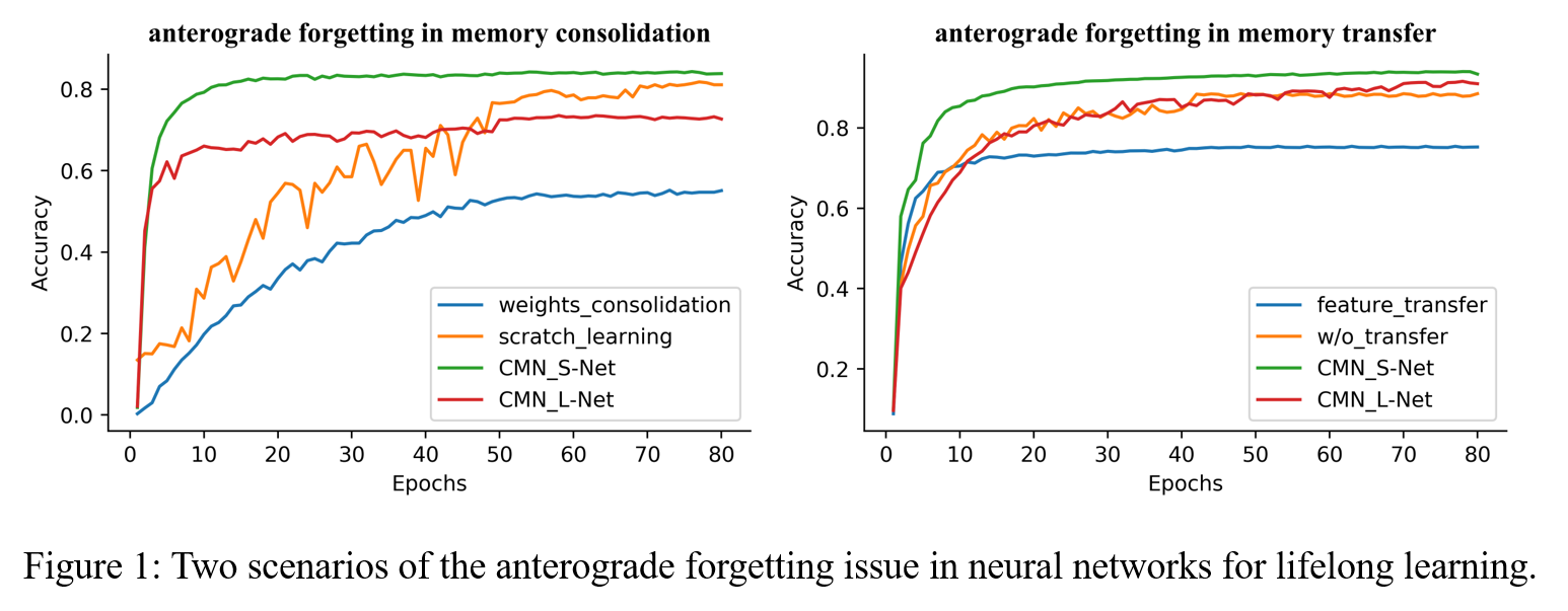
1.Anterograde forgetting

2. AF-matrics for anterograde forgetting

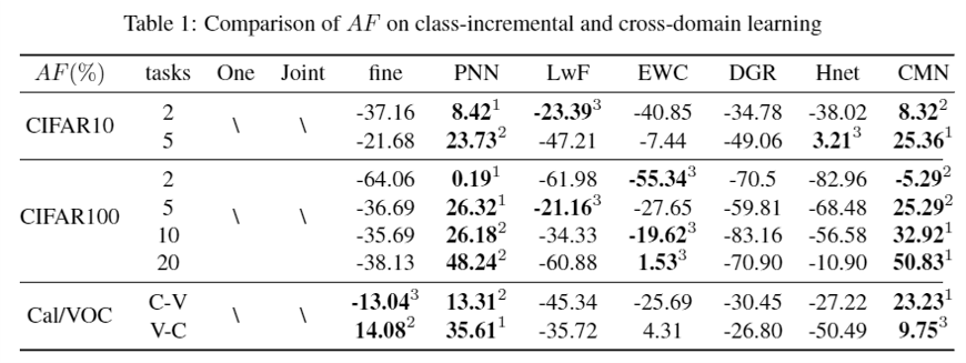
Given T task, denoting the accuracy on i-th task for the model trained on the i-th task as $P_{i,i}$ ,the average accuracy for the model trained on i task as $ACC_{i}$,the accuracy on the i-th task through the joint learning as $n_{i,i}$, and the accuracy on the i-th task through the one learning as $m_i$, AF metrics can be defined as follows： $AF= \frac{1}{T-1}\sum^T_{i=2}(ACC_{i}-n_{i,i})+\frac{1}{T-1}\sum^T_{i=2}(P_{i,i}-m_{i})$

3. BWT

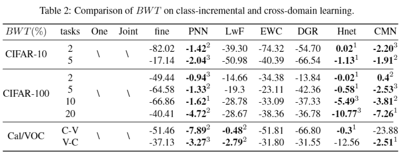
Given T task, denoting the accuracy on i-th task for the model trained on the T-th task as $P_{T,i}$ , the BWT metrics can be defined as follows: $BWT = \frac{1}{T-1}\sum_{i=1}^{T-1}(P_{T,i}-P_{i,i})$

4. Model Parameters and Iteration

The following figure shows the model parameters and iteration in 5 tasks with 20 classes for CIFAR100 experiments.

4.1.Parameters:

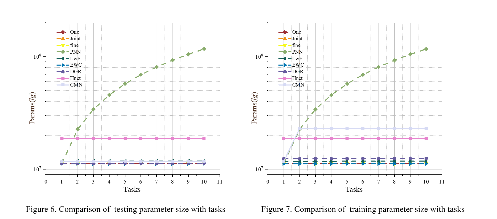
• Test Parameters: The parameters of the model in the training phase.
• Train Parameters: The parameters of the model in the training phase.

Since all method backbone are set to ResNet-18, most of the model parameters are between 10M and 20M. Among them, the model parameters of PNN reached 57M, which is because PNN generates a new sub-network for each new task as it learns, so its parametric volume reached about five times of the other model. In addition, since HNet is a hyperparametric network capable of generating weights, its parametric number also differs from other models.

Most of the models keep the same number of parameters in the training phase and the prediction phase. Since CMN requires both L-Net and S-Net in the training phase, while only L-Net needs to be used in the prediction phase, its training phase parameters are twice as many as those in the prediction phase. In addition, since DGR uses a generator for generating pseudo-images and a Solver for prediction in the training, its training phase parameters are also larger than those in the prediction phase.

4.2 Iteration Time

Iterations is the number of batches needed to complete one epoch. Denoting the number of images in a single training session as $N_p$, the Inter can be defined as:

$Iter = N_ p/batchsize$

A larger interation indicates a higher consumption of resources in a single training session. In this experiment, we have 5 tasks with 20 classes, and each class has 500 training images. And the batchsize of all methods are set to be 1024.

The number of iterations for most of the methods is equal to 10.($Iter = (500*20)/1024 = 9.765625 \approx 10$) Where Joint indicates learning all tasks at once, so it takes 50 iterations to complete an epoch. In addition, DGR will generate the same number of pseudo-images for training, so it akes 20 iterations to complete an epoch.

5. Grad CAM

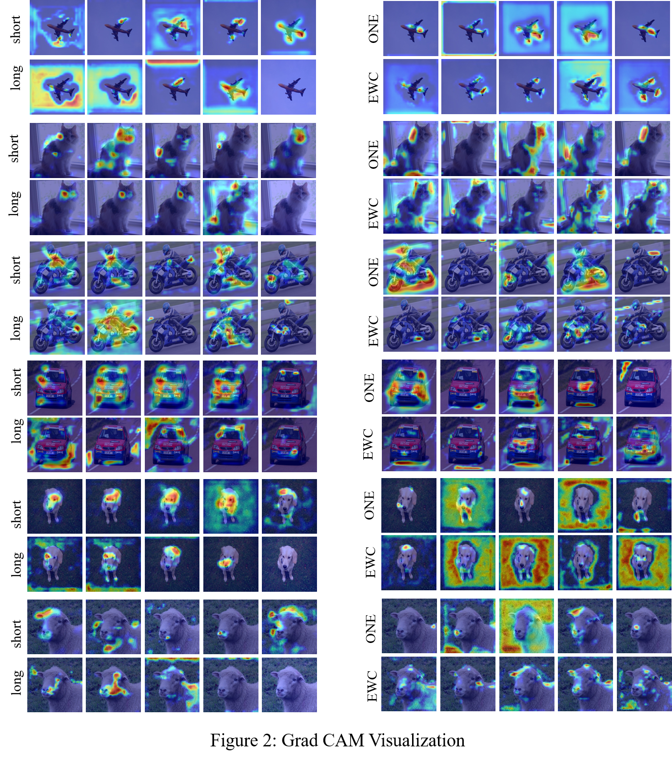
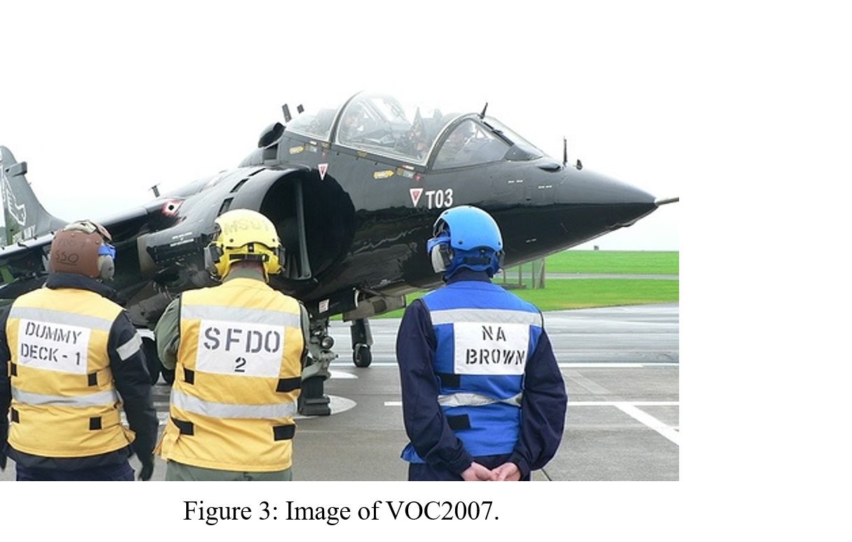
Figures 2 and 3 show all our Grad CAM visualizations. the VOC2007 dataset has a total of 20 classes of data. We selected six of these categories: cat, dog, sheep, aeroplane, car, and motorbike for visualization testing. It is worth stating that since VOC2007 is a multi-label dataset, some images have complex background information (Figure.4). Therefore, we chose images with clear backgrounds and individual objects for visualization to highlight the model learning.

6. Transfer Cell

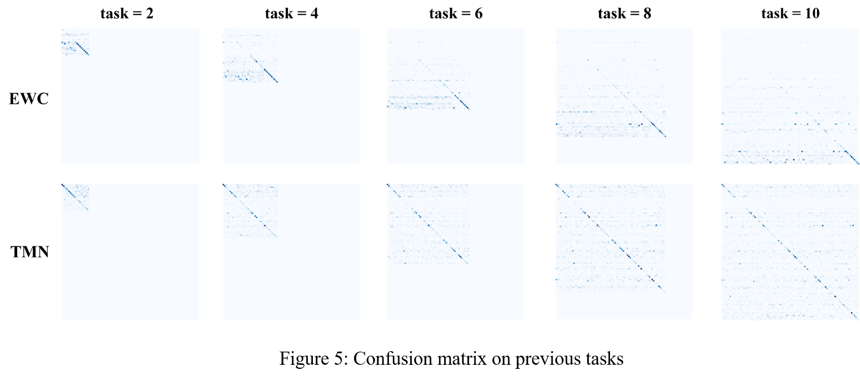
7. Confusion matrix on previous tasks

8. Statistics Analysis

We supplemented the statistics of the paper experiments. (We repeated each experiment five times.)

8.1 ACC

(The “$\backslash$” indicates that the experiment is in progress. We will keep updating the experimental data.)

8.2 FWT

(The “$\backslash$” indicates that the experiment is in progress. We will keep updating the experimental data.)

8.3 AF

(The “$\backslash$” indicates that the experiment is in progress. We will keep updating the experimental data.)

8.4 BWT

(The “$\backslash$” indicates that the experiment is in progress. We will keep updating the experimental data.)

9. Comparison of training parameter size with tasks

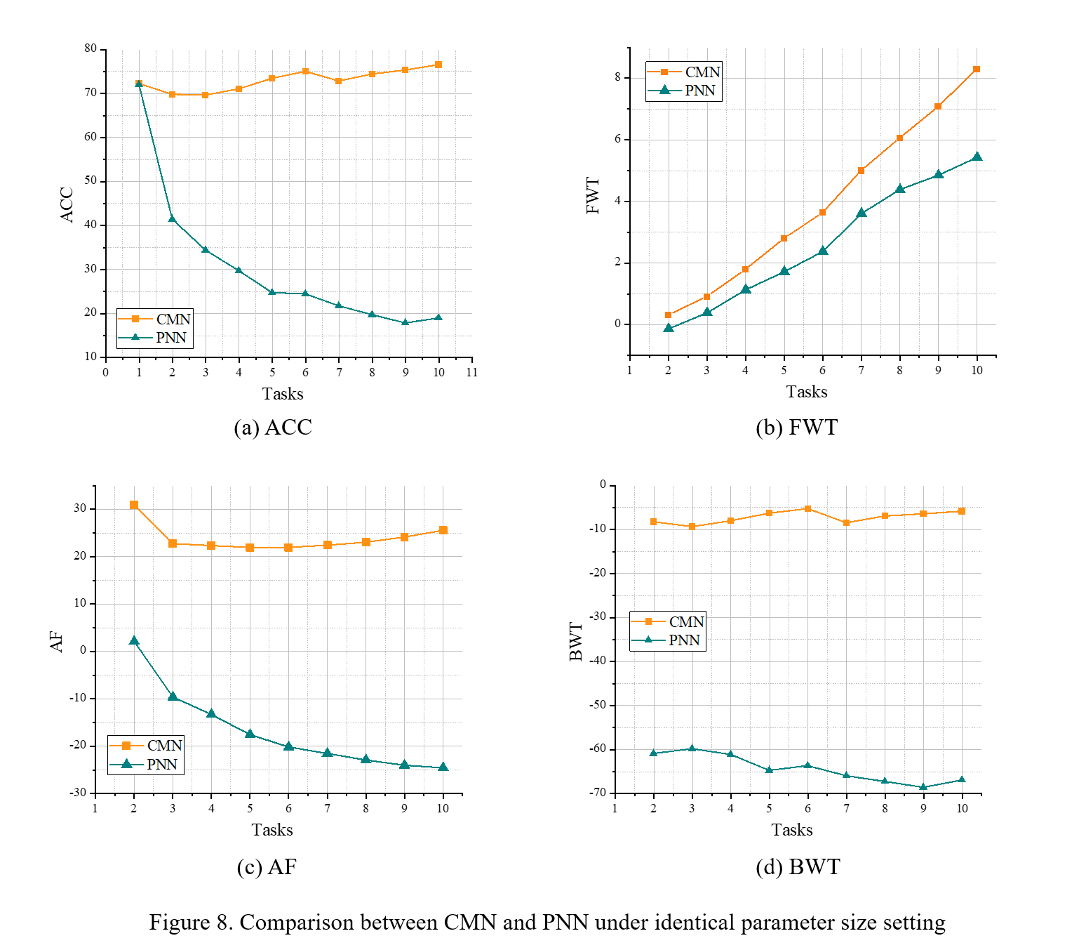
10. Comparison between CMN and PNN under identical parameter size setting

The following figure shows CMN and PNN in 10 tasks with 10 classes for CIFAR100 experiments. All methods in this part of the experiment use ResNet-18 as the backbone network.

11. Progressive Neural Networks

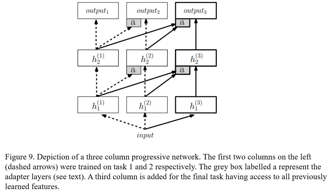
Rusu, A. A., Rabinowitz, N. C., Desjardins, G., Soyer, H., Kirkpatrick, J., Kavukcuoglu, K., … & Hadsell, R. (2016). Progressive neural networks. arXiv preprint arXiv:1606.04671.